Demographic Change, Inflation and Long-Run Asset Returns

The starting point for today's considerations is the observed high inflation, the trend reversal in the key interest rates of all central banks over the past year, and the resulting increase in nominal current yields on 10-year government bonds with negative real yields at the same time. The key question I will address today is how real interest rates may develop in the long run, from which we can infer nominal interest rates once the current high inflation phase is over (although there is, of course, a great deal of uncertainty in this respect).

For this purpose, I will use a macroeconomic simulation model, which, in the interaction of firms, households and the government sector makes statements about long-term developments, especially of per capita income as well as of interest rates. Regarding the inflation forecast, I will use a crystal ball view rather than a mathematically sound model. An optimistic – or perhaps realistic – forecast by CES-Ifo is a 2.4% inflation rate in 2024. I will assume here that the Fisher decomposition holds, i.e., that the real interest rate clears the capital market, and the inflation rate can then be added on to get the nominal interest rate. I will neglect interactions between the two objects.

The core mechanism is that capital productivity is depressed in an aging population. The reason is that capital relative to labor will be an abundant factor in an aging society. Thus, each unit of installed capital used for production of aggregate output will have a lower marginal productivity, which depresses its return. A trend reversal can occur when dissaving in an aging population more than compensates for the effects of the relative scarcity of labor, which would reduce capital formation. The macroeconomic model employed today will feature this counteracting force. Many things remain (still) unconsidered, such as the role of foreign countries and yield spreads – both of which had great weight in my earlier work – as well as the question of whether increased risk in both labor and capital income leads to an increased investment decision in fixed-income assets and thus depresses the interest rate level. Furthermore, government debt dynamics and their effects on interest rate levels (and vice versa) are not addressed.

As a central result, the model I use shows a good fit to the trajectories of real interest rates since the 1980s. The quantitative evaluation – I prefer the term quantitative evaluation, which is more tentative than, say, the term forecast –  shows low/negative real interest rates until around 2030 and then a trend reversal and a corresponding decline in the growth rate of per capita income until 2030. An important note beforehand: I neglect the time-shifted aging dynamics in other countries (the OECD is on average younger than Germany, thus aging later; the same applies to China). Taking these into account, the trend reversal in real interest rates would probably be less pronounced (see the earlier papers Börsch-Supan, Ludwig, and Winter 2006; Krueger and Ludwig 2007).

In what follows, I will first show some facts about inflation and discuss the main literature that sheds light on a link between inflation and demographics. I will then present the results of updated demographic projections for Germany and explain the core elements of the macroeconomic model. When turning to the main results, I focus exclusively on growth rates and interest rates, before finally summarizing the key messages again.

Let us first take a look at figure 1, panel (a) which shows the 12-month CPI inflation rate, i.e., the change in the price level from the previous month, shown here from January 1992 onwards. The picture shows impressively that we are currently experiencing the highest inflation since the German reunification. Let us now turn to figure 1, panel (b) which shows the CPI inflation rate since January 01, 2021. I would like to point out two main aspects. First, inflation flattened out before the Russian invasion to Ukraine, so a wait-and-see policy on the part of the ECB may have been rational during this period. In March 2022, however, we observe a sudden jump in inflation, caused in particular by energy prices, while core inflation (inflation adjusted for food and energy prices) remained largely constant at a high level and only in the last three months also recorded an increase, reaching 5.03% in November. While we see a marked decrease for the first time since March in the CPI numbers for December, the Core CPI data is not yet released. One can expect, however, that also the core CPI will continue to feature a flattening out already observed for October and November, respectively a small decrease.

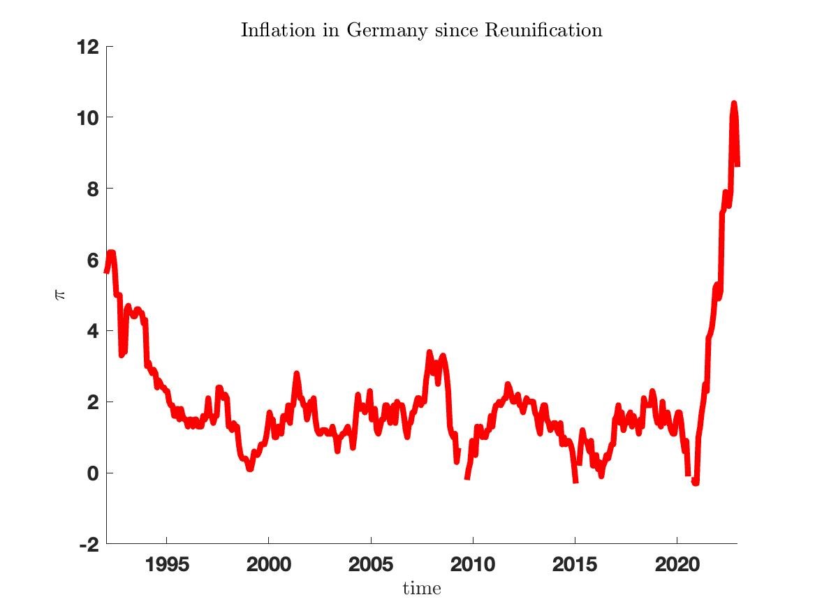
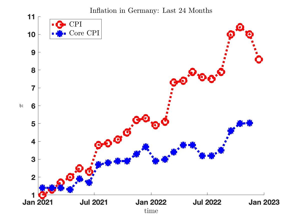
Notes: 12-mounth inflation rate in Germany. Panel (a): since 01/1992; Panel (b): last 24 months, since 01/2021.
Source: Statistisches Bundesamt, own calculations.

What can be expected? In its latest economic outlook, the German Council of Economic Experts projects a weak recovery next year and an inflation rate of 7.4%, while the CES-Ifo has it higher at 9.3% and expects a normalization and a decline to 2.4% in 2024. However, some researchers consider this forecast to be too optimistic in the medium term, as inflation has already become entrenched. Let us take a look across the Atlantic. There, too, the debate is growing louder as to whether the Fed's policy of massive interest rate hikes will hurt the economy too much. Laurence Ball, economist at the Johns Hopkins University, expects interest rates to remain high and unemployment to rise, as inflationary dynamics will remain high in the U.S. due to a depleted labor market. This which would imply a wage-price spiral, unlike perhaps in Europe, where I see more of a risk of a price-wage spiral. What makes me optimistic, despite the rise in energy prices, is an observed easing - albeit at a high level - in supply chain disruptions, falling freight costs, and falling prices for agricultural products and raw materials. We might also observe a kind of hog cycle, meaning that at least non-listed companies may have filled up inventories out of a hoarding buying motive, and thus demand for intermediate inputs will fall in some markets.

On the other hand.... If we take another closer look at the U.S., we see in Figure 2 that inflation measures that are less susceptible to fluctuations, such as median-CPI inflation - in which only prices in the middle distribution are included in the measurement - or trimmed-mean-CPI - in which prices of goods at the edge of the distribution are ignored - also show clear upward trends. So, if interest rate dynamics in the U.S. will remain or stay at a high level for a long time, this will also lead to higher interest rates in other countries due to currency devaluations. This will affect emerging markets in particular, but also the EU. Yet, also in the case of the US, the most recent data indicate that the strongest inflation dynamics might be over.

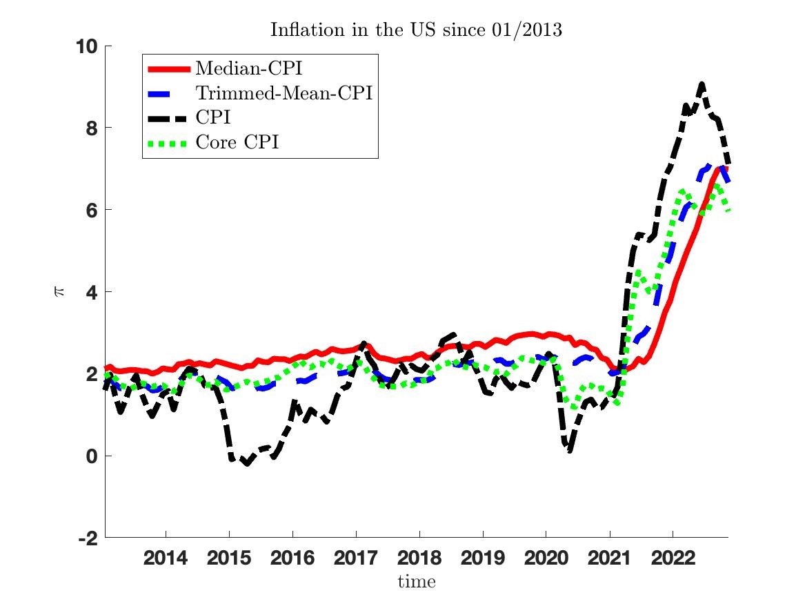
Notes: 12-mounth inflation rate in the US since 01/2013.
Source: Cleveland FED.

So there remains a high degree of uncertainty, also as far as the next question is concerned. What is the relationship between inflation and demographics? In recent years, a study by Goodhart and Pradhan (2017) on the subject has attracted a lot of attention, first concluding that demographically induced labor scarcity sets off a wage-price spiral and, second, that older people have high consumption expenditures. However, as Daniel Harenberg and I argue, Goodhart and Pradhan (2017)’s study has two fallacies. First, they use dubious consumption data. In micro data, one sees that consumption drops with age, not falls. Cruises do not have such a large weight. Second, consumption by the old must be financed, via transfers for spending on health care goods, for example, or transfers to finance income through pension systems. These transfers are made through taxes on younger ones, which dampens aggregate demand. On both aspects, see the analysis in Harenberg and Ludwig (2015, 2019) and also Brown and Ikeda (2022).

Let us next take a closer look at demographic projections. We have recently updated our population projection models used in Busch, Krueger, Ludwig, Popova and Iftikhar (2020), where we had taken an explicit focus on the effects of low skilled immigration on the German economy. According to the updated numbers and basing fertility and mortality projections on statistical models as well as assuming an annual net migration of 190 thousand per year, figure 3 shows that the population in Germany is projected to shrink over the next decades. More importantly for our succeeding analysis is, however, the evolution of the working age to population and the old age dependency ratio as shown in Figure 4. Panel (a) shows the trend shrinkage of the working age population ratio since about 1985, which will take on strong momentum over the next 20 years. Panel (b) displays the corresponding evolution of the old-age dependency ratio, which, according to our projections, is expected to increase from about 40% today to about 60% over the next 20 years, an increase by 50%.

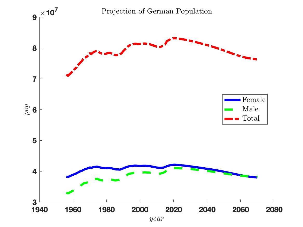
Notes: Population in Germany.
Source: Statistisches Bundesamt & Human Mortality Database, own calculations.

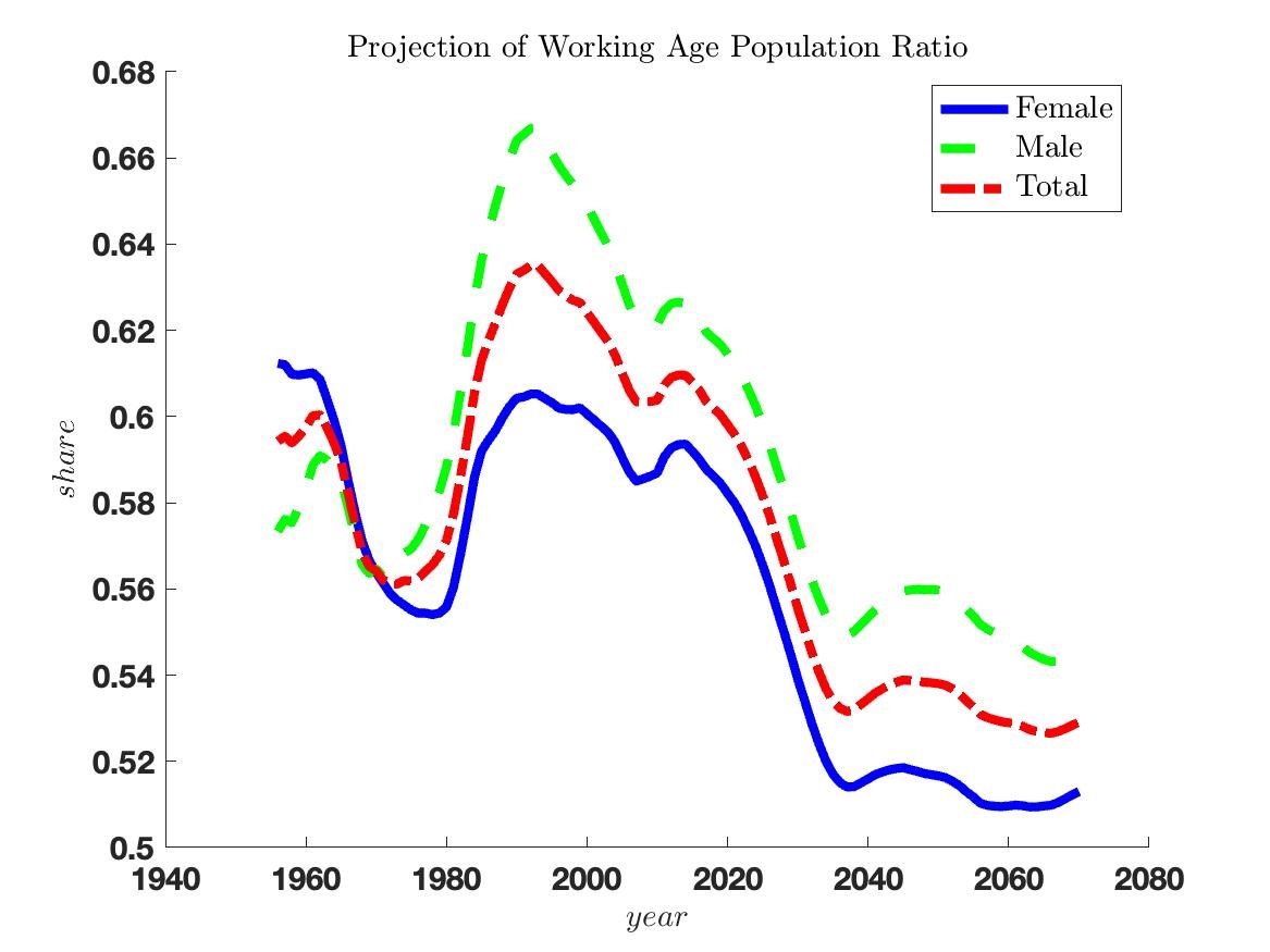
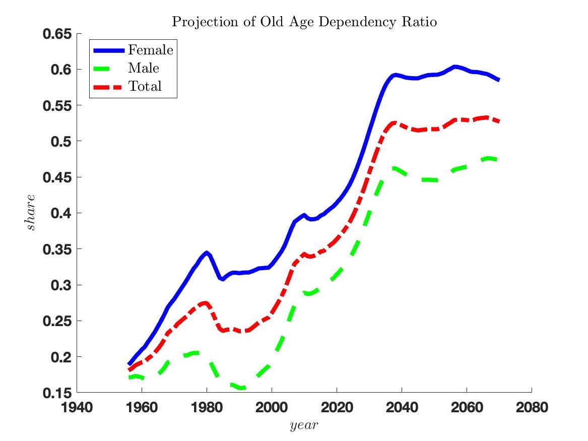
Notes: Population in Germany.
Source: Statistisches Bundesamt & Human Mortality Database, own calculations.

From a social security perspective, these trends will lead – under the maintained assumption that the German social security system will be adjusted according to the current legislation, which implies a sharing of the demographic burden among pensioners and workers – to increasing social security contribution and declining benefit rates. From a macroeconomic perspective, these trends will lead to a relative scarcity of the production factor labor and a relative abundance of the production factor capital. All else equal, this will imply a strong force towards a reduction of output and a reduction of rates of return to capital. No arbitrage across different assets implies that returns on all asset classes will be affected by this development.

Against this backdrop, I now turn to the core of my analysis, namely the evaluation of the macroeconomic effects of the projected demographic developments on two key variables of interest, per capita GDP and the risk-free rate of return sometimes also referred to as the natural rate of interest, which equalizes demand and supply on the capital market. I want to reemphasize that the following analysis is neither a forecast nor a prediction but rather a quantitative evaluation of the likely effects of a specific mechanism. To model it, I develop a complex quantitative overlapping generations model with firms that optimize production plans employing capital and labor as inputs and households that optimize their consumption savings plans in the course of a life cycle. Exogenous to the model are the demographic developments and, as already stated in the introduction, in the current analysis the sole role of the government is the organization of a PAYG pension system and any interactions with foreign countries are ignored.

Out of the model parameters that are taken as exogenous, I want to emphasize two-time varying parameters that in addition to the demographic processes are used as inputs in the model. The time paths of both these parameters are displayed in Figure 4. In the figure, the red dashed line displays the smoothed growth rate of the so-called Solow-Residual. It is the growth rate of technology, which is computed as the component of real aggregate output (GDP) of a country, which cannot be attributed to the measured real aggregate capital stock and the aggregate hours worked. The figure shows a clear productivity slowdown since 1965. Importantly, it is not only since the Great Recession in 2008/09 that the Solow-Residual displays low growth in Germany of around 0.5% annually relative to a long-run OECD average of 1.5%. Rather, such low growth can be observed since about year 2000. Through the lens of the quantitative model employed here for prediction of future returns, low growth suppresses returns through two channels. First, it reduces returns directly because the marginal product of each unit invested is lower if the investment depreciates faster. Second, it also reduces returns indirectly because it reduces the efficiency of units of labor employed in production and thus the capital stock relative to productive labor becomes even more abundant.

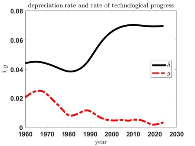
Notes: Solow residual (red dashed line) and depreciation rate (black solid line) on capital in Germany. Trend component. Original data are smoothed with Hodrick-Prescott filter using a standard penalty parameter on the cyclical component of 100.

Source: AMECO, own calculations.

The black solid line in Figure 4 in turn shows the smoothed depreciation rate of capital since the 1960s, which has increased over the past decades reflecting that in modern societies apparently the installed level of capital becomes obsolete at a faster rate. Through the lens of the quantitative model employed here for prediction of future returns, this has two partially offsetting implications. On the one hand side, higher depreciation reduces returns directly. On the other hand, higher depreciation in one period means that the capital stock is lower in the next period reducing the relative abundance of capital. 

I now turn to a backfitting analysis of the model. Computational simulations of the equilibria on the markets for output, capital and labor start in year 1955, but are subject to initialization assumptions. We therefore look at outcome variables only 30 years after this initial date so that initialization assumptions do not affect the outcome much. The left-hand side of Figure 6 shows the model simulated time path of per capita GDP. The blue solid line is the data, and the red dashed line gives the model output under a baseline simulation where the long run trend growth rate of technology is set to g=0.5%, on the basis of the data presented in figure 5. Overall, while getting the trend right, the model slightly overshoots the decline of the growth rate. The model does also not capture the significant blip in the trend growth rate around 1991 – there is no German reunification shock in the model. The other two lines in the figure show two counterfactual simulations intended to decompose the trend growth into its component. It shows that about 60% of the reduction of the GDP per capita growth rate can be attributed to demographic developments (violet line). Panel (b) shows the real interest rate in the model and compares it to the corresponding smoothed data series. The model does not match the full decline in the risk-free interest rate (the return on 10-year government bond yields): it predicts a decline over the period of -4.5%p whereas the actual decline was -6.3%p. Through the lens of the model, about 20% of this decline can be attributed to the demographic development, i.e., 1%p.

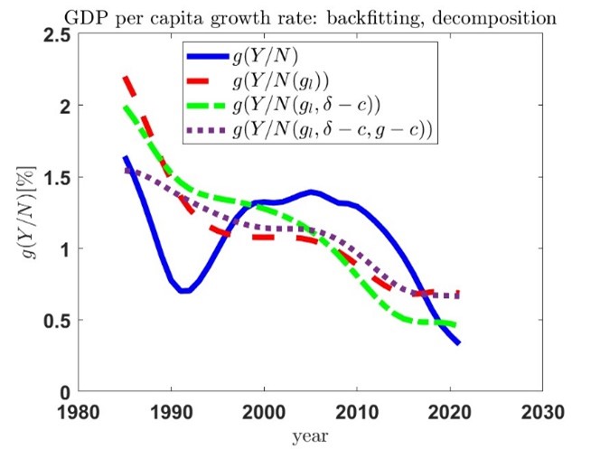
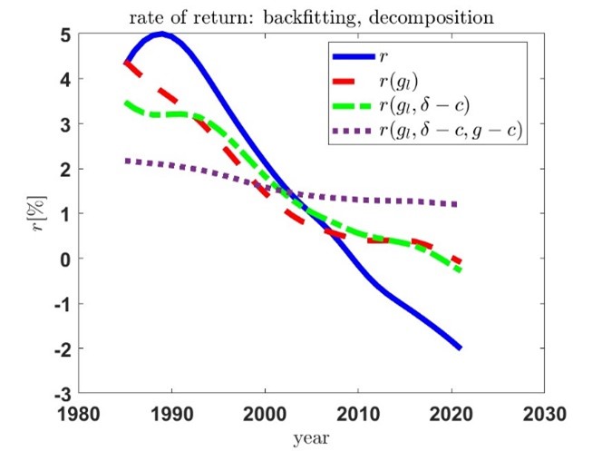
Notes: Panel (a): Per capita GDP growth rate. Panel (b): risk-free real rate of return (10-year government bond yields). Blue solid line: data. Red dashed line: model (baseline scenario). Green dashed-dotted line: model assuming constant deprecation rate. Purple dotted line: model assuming constant deprecation rate and constant rate of technological progress.

Source: AMECO, EIOPA (2022), own calculations.

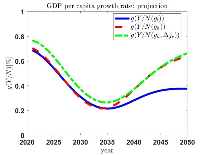
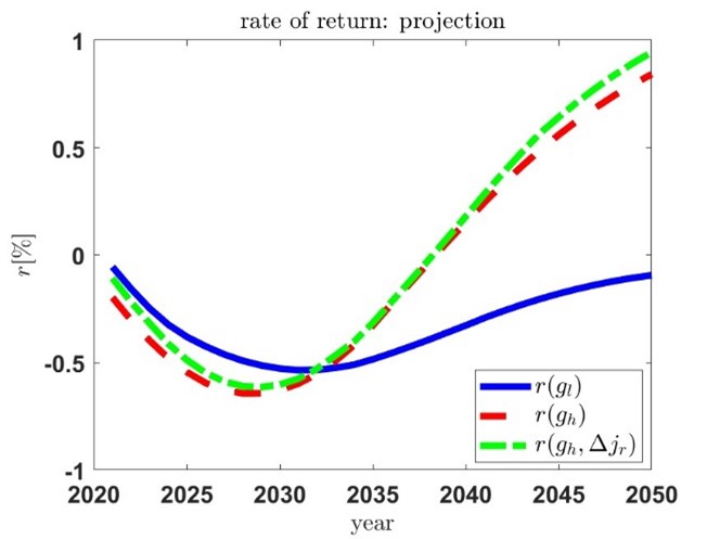
Notes: Panel (a): Per capita GDP growth rate. Panel (b): risk-free real rate of return (10-year government bond yields). Blue solid line: model (baseline scenario). Red dashed line: model assuming higher rate of technological progress. Green dashed-dotted line: model, additionally assuming increasing retirement age.

Source: AMECO, own calculations.

Finally, we turn to the model predictions. As shown in panel (a) of figure 7 the model predicts a reduction of the trend growth rate of GDP per capita by about 0.5%p until 2035 and a rebound thereafter. Assuming a stronger productivity trend growth rate of 1% (instead of 0.5% as we do in the baseline) does not help the economy to avoid the size of the reduction but leads to a stronger increase after the trough. Finally, an increase in the retirement age somewhat stabilizes the reduction in the growth rate of output per capita. This rebound effect is even stronger for the rate of return, shown in panel (b) of the figure. Somewhat surprisingly, the higher rate of technological progress only shows pronounced effects after the coming demographic wave fades out. Also, note that the effects of increasing the retirement age on per capita income growth basically leads to a level shift (it leads to a level shift of output) and can thus attenuate the effects on long-run growth, but the effects are mild, particularly on the rates of return.

I draw the following three main conclusions. Frist, the persistent low interest environment – which according to the above quantitative evaluation will continue for decades into the future – calls for retirement investments in stocks and other risky assets instead of relying heavily on fixed interest investments. While out of a no arbitrage argument, rates of return on risky investments will also fall in the demographic change process (cf. Abiry, Geppert and Ludwig 2016), they deliver a positive return differential over the long run. In contrast, any form of rate of return guarantee in insurance products – which forces the provider to invest in low risk, low return assets – is a real expropriation of an investor’s wealth. Second, if we follow this path of increased investments in risky assets to fund pensions in individual accounts, this will lead to horizontal equity concerns because while stocks pay out high returns in the long run, return histories may fluctuate strongly across subsequent cohorts retiring and annuitizing their wealth in retirement. This brings us back to the Feldstein and Samwick (1992, 1999, 2000) proposal, also see Ball and Mankiw (2007), according to which we need public-private partnership design in pension systems by a compensation scheme through public pensions and taxation that may be adjusted to smooth out such income fluctuations (and may be financed using government debt). Third, we need to understand better the relationship between demographic change and technological progress, both theoretically and empirically. The analyses in Ludwig, Schelkle and Vogel (2012), Heer and Irmen (2014) and Acemoglu and Restrepo (2017) provide natural starting points for such an investigation.

Acemoglu, D. and P. Restrepo (2017). Secular Stagnation? The Effect of Aging on Economic Growth in the Age of Automation. American Economic Review 107 (5), 174- 179.

Ball, L. and N. G. Mankiw (2007). Intergenerational Risk Sharing in the Spirit of Arrow, Debreu, and Rawls, with Applications to Social Security Design. Journal of Political Economy 115(4), 523-547.

Börsch-Supan, A., A. Ludwig and J. Winter (2016). Ageing, Pension Reform and Capital Flows: A Multi-Country Simulation Model. Economica 73(292), 625-658.

Brown, A.R. and D. Ikeda (2022). Why Aging Induces Deflation and Secular Stagnation. Working Paper.

Busch, C., Z. Iftikhar, D. Krueger and I. Popova. Should Germany Have Built a New Wall? Macroeconomic Lessons from the 2015-2018 Refugee Wave. Journal of Monetary Economics 113(C), 28-55.

Feldstein, M. and A. Samwick (1992). Social Security Rules and Marginal Tax Rates. National Tax Journal 45(1), 1-22.

Feldstein, M. and A. Samwick (1999). Maintaining Social Security Benefits and Tax Rates Through Personal Retirement Accounts: An Update Based on the 1998 Social Security Trustees Report. NBER Working Paper No. w6540. Available at: papers.ssrn.com/sol3/papers.cfm

Feldstein, M. and A. Samwick (2000). Allocating Payroll Tax Revenue to Personal Retirement Accounts to Maintain Social Security Benefits and the Payroll Tax Rate. NBER Working Paper No. w7767. Available at: papers.ssrn.com/sol3/papers.cfm

Geppert, C., A. Ludwig and R. Abiry (2016). Secular Stagnation? Growth, Asset Returns and Welfare in the Next Decades: First Results. SAFE Working Paper No. 145. Available at: papers.ssrn.com/sol3/papers.cfm

Goodhart, C. and M. Pradhan (2017). Demographics will reverse three multi-decade global trends. BIS Working Papers No. 656. Avaiable at: www.bis.org/publ/work656.pdf

Harenberg, D. and A. Ludwig (2015). Social Security in an analytically tractable overlapping generations model with aggregate and idiosyncratic risks. International Tax and Public Finance 22(4), 579-603.

Harenberg, D. and A. Ludwig (2019). Idiosyncratic Risk, Aggregate Risk, and the Welfare Effects of Social Security. International Economic Review 60(2), 661-692.

Heer, B. and A. Irmen (2014). Population, Pensions, and Endogenous Economic Growth. Journal of Economic Dynamics and Contral 46(C), 50-72.

Krueger, D. and A. Ludwig (2007). On the consequences of demographic change for rates of return to capital, and the distribution of wealth and welfare. Journal of Monetary Economics 54(1), 49-87.

Ludwig, A., T. Schelkle and E. Vogel (2012). Demographic Change, Human Capital and Welfare. Review of Economic Dynamics 15(1), 94-107.